Assignments

5th Assignment

Due: Mon 4 May

Warm-up Task

Look back at the writing reflection you submitted with your 1st Assignment: The paragraph identifying a major error in your math writing and the steps you planned to take.
- Quote or paraphrase what you wrote then. Has the improvement you described actually happened? Provide a brief “before” excerpt (from any of your earlier assignments this semester) and an “after” excerpt (from more recent work) as evidence.
- Identify one new issue in your technical writing that you have only recently become aware of (i.e., something you did not notice at the start of the semester). This could be a strength you now want to push further, or a weakness that earlier problems were too simple to expose.
- Keep this reflection to one well-crafted paragraph; precision and self-awareness matter more than length.

Main Task: Choose Your Own Adventure

Your assignment is to solve some of the exercises from the interactive lessons on feedforward networks, backpropagation, deep network architectures, and generative models. You do not need to solve every exercise: That is too much to ask! Instead, this is a “choose your own adventure” assignment: Choose exercises that interest you and that push your understanding.

Format requirements are the same as for the 4th Assignment: typeset in LaTeX at 12pt, single-spaced, 1 in. margins, using the provided LaTeX Homework Template.

Your submission should be at least 4 pages (excluding the warm-up) and include at least two figures, drawn from at least two different lessons below. You are allowed to use AI to generate figures as long as you include the exact prompt used; a vague prompt such as “make a figure about backpropagation” will not receive full credit.

You must complete (some) exercises from at least three different subtasks I–IV below.

Subtask I: Units, Activations, and the Forward Pass

Open the Forward Pass & Activation Functions lesson in Colab and follow it through. Choose and solve some of the exercises listed in Sections §2 and §4:

Exercise 2.1 (Linear networks collapse): Extend the two-layer linearity check to $L = 5$ layers; analyze a non-identity linear activation; state what the Universal Approximation Theorem says.
Exercise 4.1 (Counting parameters): Derive the general parameter-count formula; apply it to the MNIST architecture; compare widths 64 vs. 128.
Exercise 4.2 (Choosing activations): Justify the correct output activation for single-label classification, multi-label detection, and regression.
Exercise 4.3 (Vanishing gradients: Experiment): Run the gradient-norm scaffold with sigmoid and ReLU; explain the difference; find an initialization scale that stabilizes sigmoid.

Subtask II: Backpropagation

Open the Backpropagation lesson in Colab. Choose and solve some of the exercises in Sections §3–§5:

Exercise 3.1 (Chain rule on the graph): Verify $\partial\ell/\partial w$, $\partial\ell/\partial b$, $\partial\ell/\partial x$ by hand; redo the backward pass for a sigmoid unit; explain why large-magnitude inputs lead to large weight updates.
Exercise 4.1 (Deriving $\delta^{(L)}$): Derive the output-error formula $\delta^{(L)} = \hat{\mathbf{y}} - \mathbf{y}$ from the softmax and cross-entropy expressions.
Exercise 4.2 (Hidden-layer recurrence): Fill in the full derivation of $\nabla_{W^{(l)}}\mathcal{L} = \delta^{(l)}(\mathbf{a}^{(l-1)})^\top$; interpret the ReLU backward pass in terms of dead units.
Exercise 5.1 (Extending to a batch): Generalize the forward/backward code to a batch of $B$ examples; verify that one gradient step decreases the loss.
Exercise 5.2 (Sigmoid network): Swap ReLU for sigmoid, re-run the gradient check, and compare $\delta^{(1)}$ magnitudes between the two activations.

Subtask III: Deep Network Architectures

Open the DNN Architectures Overview in Colab. Follow the lesson through its survey of MLP, CNN, RNN, Transformer, and autoencoder families, and complete exercises of your choice. As a guide, here are the kinds of questions worth addressing:

Compare the parameter count and inductive biases of a fully-connected layer vs. a convolutional layer of similar “capacity.”
Explain, in your own words, why a recurrent network can in principle process sequences of arbitrary length, while a fixed-window feedforward network cannot.
Describe the self-attention mechanism: What are queries, keys, and values, and how does the scaled dot-product formula produce an attention matrix?
Explain the role of the encoder and decoder in an autoencoder; contrast a plain autoencoder’s latent space with that of a VAE (connecting to Subtask IV below).

Subtask IV: Generative Models

Open the Generative Models lesson in Colab. The exercises are listed at the end of the notebook (Section §7); choose and solve some of them:

ELBO derivation: Use Jensen’s inequality to derive the ELBO; show that the gap equals $ D_{\mathrm{KL}}(q_\phi(\mathbf{z}|\mathbf{x})|p_\theta(\mathbf{z}|\mathbf{x})) $.
KL weight experiment: Train the VAE with kl_weight values 0.01, 0.1, 1.0, 10.0; visualize and explain the reconstruction vs. regularization tradeoff.
Temperature and entropy: Prove that the entropy of the temperature-scaled softmax is monotone in $\tau$; verify empirically.
Autoregressive generation speed: Compare generation cost (forward passes) between autoregressive models and VAEs; discuss quality tradeoffs.
PCA vs. VAE on the circle: Explain why a 1-D VAE latent space is topologically insufficient for the circle; determine the minimum latent dimension for a torus (surface of a doughnut).

4th Assignment

Due: Wed 15 April

Warm-up Task

Identify one area of strength as technical writer where you have grown this semester, as well as one area of weakness.
- Give an example of “before” (how you would have written an explanation at the beginning of the semester; it can be a sample of your actual writing) and “after” (how you would write it now).
- Give also an example of what still “needs work” based on a recent sample of your writing that, based on our Writing Guidelines.

Main Task: Choose Your Own Adventure

Your assignment is to solve some of the exercises and problems in the interactive lessons on the Bias-Variance Tradeoff and Stochastic Gradient Descent. You do not need to solve and turn in all the problems and exercises —that is a little too much to ask! Instead, this is a ”choose your own adventure” assignment. Make sure it is typeset in LaTeX at 12pt, single-spaced, 1 in. margins (you may simply use the provided LaTeX Homework Template. (To compile the mock template without errors, you need also the figure (PNG file).)

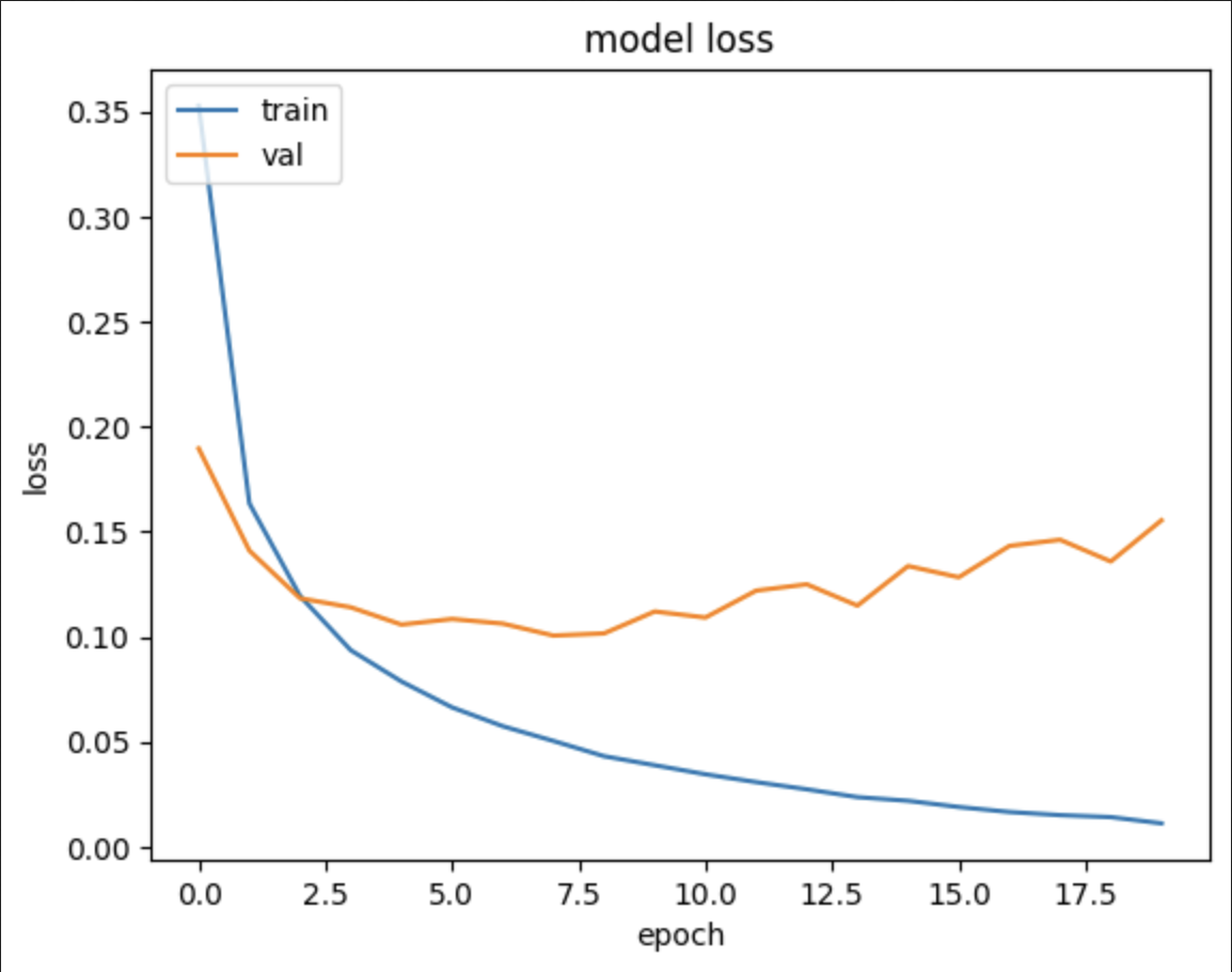
Your submission should be at least 4 pages long, and include at least two figures, one related to the material of each lesson. You are allowed to use AI to generate the figures as long as you provide (i.e., include in the document) the prompt/query used to generate it; the prompt should be specific, thoughtful and well posed. (A very simple prompt such as “make a figure related to problem #7” will result in a very generic image that will not receive a good grade.)

Subtask I

Open the Bias-Variance Tradeoff Lesson in Colab. Follow the lesson along. Choose and solve some of the exercises at the end (in Section §9).

Note: This lesson uses the scikit-learn (“sklearn”) Python framework, which is a learning tool simpler than any of the frameworks (such as Keras/PyTorch/Tensorflow/JAX) used for industrial and research work. (Our old friend Keras is still used in the lesson, too.)

Subtask II

Do the same for the lesson on Stochastic Gradient Descent. Follow the lesson along and solve some exercises of your choice.

Optional Subtask III

If you want to start working on material for the next assignment, here is a link to the overview of deep network architectures. However, do not turn in any problems from this material.

3rd Assignment

Due: Wed 4 March

Warm-up Task

(Re)read the Written Work Guidelines and write a short paragraph reflecting on your progress as a technical writer. Be specific; show that you understand your areas of strength and weakness better than you did at the beginning of the semester.

Task I

Refer to the discussion of multivariate normal random variables (normally distributed random vectors) in §3.3, and also to the Multivariate Normal Primer by @peterroelants. You may and should use other resources in completing this task; high-quality reference textbooks are encouraged.

Consider an arbitrary n×n real matrix A. The n×n matrix $S = A^{\top} A$ is real symmetric and positive semi-definite. (S is positive definite when its rank is exactly n.) Therefore, S is a valid covariance matrix for an n-multivariate normal distribution; in fact (apart from possible zero eigenvalues), the eigenvalues of S are the squares of the singular values of A, and the eigenvectors of S are the right-singular eigenvectors of A.

Write at least one full page explaining the precise relationship between the SVD of A and the ellipsoidal level curves of the normal PDF with covariance matrix S. At the very least, your explanation should explain what are the exact directions and lengths of the (principal) axes of the ellipsoid with equation \[ \mathcal{N}(\mathbf{x}) = \exp\bigl(-Q(\mathbf{x})\bigr)/\sqrt{(2\pi)^n\det(S)} \] where the positive semidefinite quadratic form $Q(\mathbf{x}) = (1/2)\mathbf{x}^\top S^{-1} \mathbf{x}$.

Bonus subtask A

What goes wrong if A —and therefore also S— is a singular matrix?

Task II

Subtask A

Let $\mathcal{N}$ be the standard normal distribution $\tilde{\mathcal{N}} = \mathcal{N}_{\mu,\sigma}$ be the normal distribution with mean $\mu$ and standard deviation $\sigma$. Evaluate the (Kullback-Leibler) KL-divergence $D_\mathrm{KL}(\mathcal{N}\parallel\tilde{\mathcal{N}})$ in closed form.

Hint: Besides algebraic manipulations, all you should need are the values $\int_{-\infty}^{+\infty}\mathcal{N}(x)dx = 1$, $\mathbb{E}(X) = \int_{-\infty}^{+\infty}x\mathcal{N}(x)dx = 0$ and $\mathbb{E}(X^2) = \int_{-\infty}^{+\infty}x^2\mathcal{N}(x)dx = 1$.

For the remaining subtasks, let $B_p$ be the PDF of a Bernoulli random variable with parameter $0\le p\le 1$, i.e., $B_p(1) = p$, $B_p(0) = 1-p$ (and $B_p(x) = 0$ for $x\ne 0, 1$).

Below, we assume $p,q\in[0,1]$, i.e., the pair $(p,q)$ belongs to the unit square $[0,1]\times[0,1] = [0,1]^2$.

Subtask B

Evaluate the KL divergence $D_{\mathrm{KL}}(B_p\parallel B_q)$ in closed form (i.e., give a formula), and verify that $D_{\mathrm{KL}}(B_p\parallel B_{1-p}) = D_{\mathrm{KL}}(B_{1-p}\parallel B_p)$. Can you provide a conceptual explanation of the meaning of this equality?

Optional Subtask C

Describe the regions of the unit square consisting of points $(p,q)$ where, respectively

$D_{\mathrm{KL}}(B_p\parallel B_{q}) < D_{\mathrm{KL}}(B_{q}\parallel B_p)$;
$D_{\mathrm{KL}}(B_p\parallel B_{q}) = D_{\mathrm{KL}}(B_{q}\parallel B_p)$;
$D_{\mathrm{KL}}(B_p\parallel B_{q}) > D_{\mathrm{KL}}(B_{q}\parallel B_p)$. (Your description of those regions should be precise, but not necessarily be backed by formal proof —which will be messy.

An answer/conjecture found using numerical exploration/graphing is acceptable.)

2nd Assignment

Due: Wed 18 February

Warm-up Task

(Re)read the Written Work Guidelines and write a short paragraph reflecting on your progress as a technical writer.

Main Task I

Log on to Colab and open the Jupyter (iPython) file numpy-tutorial-svd.ipynb.

Make sure to save it to your own Google Drive! (The link above is to a read-only version of my personal copy of the file). Afterwards, you should continue work on your own personal copy.

Take a “random” 3×2 matrix A of your own choosing meeting the following requirements:

it has small integer entries, say 0, ±1, ±2, ±3 (repetitions are allowed, and you are also allowed to use larger integers but the calculations may get messier);
it has rank 2;
no two rows, nor columns should be perpendicular;
at most two entries are zero, but not in the same row nor column.

Subtask 1 [50 pt.]

Run through the entire calculation of finding the Singular Value Decomposition of A.

Your calculations should all be exact —not decimal approximations. Square roots are almost certain to be involved in computing eigenvalues and entries of eigenvectors. Do not evaluate those numerically, but do simplify the exact expressions as much as possible (e.g., although square roots of relatively large integers may appear, at no point should you have a square root nested inside another one, etc.)

The steps are as follows:

Consider first the 2×2 matrix $B = A^{\top}A$. Carry out in full all steps for finding the (positive!) eigenvalues $s_1$, $s_2$ (chosen in the decreasing order of magnitude $s_1 > s_2$) and an orthonormal basis $v_1$, $v_2$ (ONB) of eigenvectors of B —these are the “right eigenvectors” of A.

The eigenvalues $s_1 > s_2$ of B are the “squared singular values” of A. The singular values of A are thus defined as $\sigma_1 = \sqrt{s_1}$ and $\sigma_2 = \sqrt{s_2}$.

The ONB $v_1$, $v_2$ gives (the columns of) an orthogonal 2×2 matrix $V$. Verify that $V^\top V = I$.

Consider now the 3×3 matrix $C = AA^{\top}$. Carry out all steps of finding the eigenvalues and an orthonormal basis $u_1$, $u_2$, $u_3$ (ONB) of eigenvectors for C—these are the “left eigenvectors” of A. Verify that the corresponding eigenvalues should be $s_1$, $s_2$ (which are the same squared singular values of A as above) and the third eigenvalue is $0$. The ONB $u_1$, $u_2$, $u_3$ gives (the columns of) an orthogonal matrix $U$. Verify that again $U^\top U = I$.
Let Σ be the 3×2 matrix (same size as A) having the singular values $\sigma_1$, $\sigma_2$ on the diagonal. Verify that \[ \sigma_1(u_1v_1^\top) + \sigma_2(u_2v_2^\top) = A = U\Sigma V^\top. \]

Subtask 2 [25 pt.]

Find numerical approximations (using a calculator or Python/NumPy) to the matrices U, S, V you found above, and write them down.
Use NumPy to find (a decimal approximation to) the SVD of the same matrix A chosen above. (Hint: Use NumPy’s function linalg.svd as done in numpy-tutorial-svd.ipynb. Remember to start with import numpy as np so you can subsequently access the function as np.linalg.svd.)
Do the matrices U, S, V you found in (i) above answer agree exactly (to within a small rounding error) with the ones found using linalg.svd? How many different choices of the matrix triple (U, \Sigma, V) are possible, all of which are equally correct as an SVD for A?
[Bonus +5%] Count the possible choices of (U, \Sigma, V) for a given matrix A still of rank 2, but having size 4×2.

Subtask 3 [25 pt.]

As in Cell #25 of numpy-tutorial-svd.ipynb, let k be any positive integer not exceeding 768, which is the rank, in all likelihood exact, of the “raccoon matrix” img_gray. In numpy-tutorial-svd.ipynb, only the largest k = 10 singular values (out of 768) are kept, providing a “lossy”/blurry reconstruction of the original image which, remarkably, is still quite recognizable as a raccoon. Carry out experiments varying the value of k and report your findings. What is the smallest value of k for which there is no visually discernible difference between the original picture and the reconstructed one?

Although computing the SVD of a very large matrix is quite an expensive operation for which no truly efficient algorithm is known, the notions of “encoder/decoder” in modern machine learning (deep neural networks) are inspired by (but not based on) optimal/ideal mathematical procedures such as SVD.

Bonus subtask 4 [15 pt.]

Read about the relation between SVD and PCA (Principal Component Analysis) in section §2.12 of the textbook and (at least one) additional source(s). Write a summary —with illustration(s)!— of your findings and spanning at least a half-page.

1st Assignment

Due: Wed 4 February

Warm-up Task

Read the Written Work Guidelines and documents on mathematical writings referenced therein. Write a short paragraph (≈5 lines) reflecting on one major error present in your math writing hitherto, and outlining some steps you will take to improve your writing for this course. Each written assignment throughout the semester should start with a short 1-paragraph reflection on a different issue you have noticed, and outline steps to address it. (You will need to continuously revisit the Written Work Guidelines and documents therein referenced.)

Task I

Open the Jupyter (iPython) notebook intro_feedforward_mnist.ipynb (link opens the notebook in Google Colab) which creates and trains a simple feedforward-network to learn to recognize handwritten digits in the MNIST “database”—which is more of a dataset than a database as such.

Make sure to look at the MNIST Wikipedia page and Figure 1.9 in Deep Learning Ch. 1.

Make sure to Save your own personal copy of the file (e.g., to your Google Drive).
- You cannot save it back to Github (not authorized).
Although the Python code is somewhat complicated, it has many comments. There are also a couple of parameters whose numerical value you can adjust interactively (but you must re-run notebook cells for those changes to take effect).

Sub-Task 1

Play around assigning different values to the parameters dim_hl_1, dim_hl_2 (dimensionalities of the 1st and 2nd hidden layers) and the number num_epochs of epochs. Make a table and provide a human-readable analysis of your findings.

For extra credit +20%, also compare the 2-hidden layer feedforward NN to NNs with 1 or 3 hidden layers. (You will need to make minor edits to the code in intro_feedforward_mnist.ipynb.)

Sub-Task 2

There are probably at least a few new and unfamiliar concepts present in or implied by the code. Choose one aspect or issue you would like to understand better, research it, and write about 1 page summarizing your findings. This sub-task requires you to analyze and explain (not simply cut-and-paste content). Examples include (but are not limited to):

What is a TPU? What are its similarities and differences to a CPU and a GPU?
What is Keras? What is Jax? What is NumPy? How are they related?
What is a float32 precisely? How are those 32 bits used to store real numbers?
What other kinds of floats and numerical types does NumPy support?
What does a Keras model actually consist of? What does it look like as a Python object?
What is a “logit”? What is a “ReLU”? What is “categorical cross-entropy”?
What are other datasets beyond MNIST broadly used as NN benchmarks?
What is the difference between training, validation and test datasets?
What is the difference between a feedforward network and other kinds of neural networks?
What is root mean-square propagation? How does it compare to other optimization methods?
What part of the code in intro_feedforward_mnist.ipynb do I find most mysterious? Can I try to better understand and explain what it’s doing?